Music separation with DNNs: making it work
fabian-robert.stoter@inria.fr
faroit
antoine.liutkus@inria.fr
September 23rd, 2018

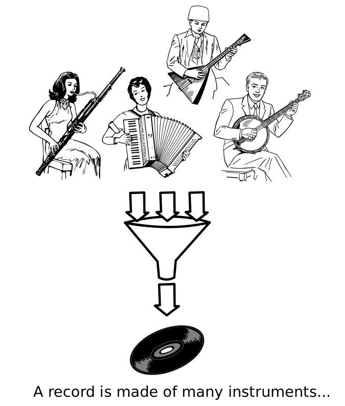
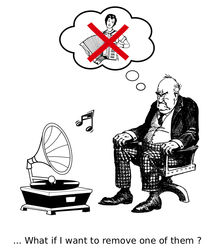
Music Unmixing/Separation
Applications
- Automatic Karaoke
- Creative Music Production
- Active listening
- Upmixing (stereo $\Rightarrow$ 5.1)
- Music Education
- Pre-processing for MIR
Motivations
- Intense past research
- Many evaluation campaigns: MIREX, SiSEC
- Recent breakthroughs: separation works
- Difficult topic
- Signal processing skills
- Deep learning experience
- Objectives of this tutorial
- Basics of DNN, basics of signal processing
- Understand an open-source state of the art system
- Implement it!

Tutorial outline
- Introduction
- Our vanilla model
- Choosing the right representation
- Tuning the DNN Structure
- Training tricks
- Testing tricks
- Conclusion
Outline
Introduction
- Time-frequency representations
- Filtering
- A brief history of separation
- Datasets
- Deep neural networks
Mixture spectrogram
Vocals spectrogram
Drums spectrogram
Bass spectrogram
Introduction: time-frequency representations
Hands on
- Start the notebook session
- For one track, display waveforms, play some audio
- Display spectrogram of mixture
Introduction: time-frequency representations
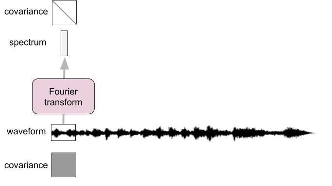
Spectral analysis as pre-whitening

- Frames too short: not diagonalized
- Frames too long: not stationary
Introduction: time-frequency representations
Spectral analysis as pre-whitening
Introduction: filtering
Hands on
- Get spectrograms of the sources
- Display the corresponding soft-mask for vocals
- Apply it on the mixture, reconstruct and listen to the result
Introduction: filtering

Introduction: filtering

Introduction: filtering

Introduction: filtering

Introduction: filtering


Introduction: filtering

Introduction: a brief history
The big picture

Rafii, Zafar, et al. "An Overview of Lead and Accompaniment Separation in Music." IEEE/ACM Transactions on Audio, Speech and Language Processing (TASLP) 26.8 (2018): 1307-1335.
A brief history: model-driven methods
Harmonicity for the lead

- Pitch detection
- Clean voices
- "Metallic" artifacts
A brief history: model-driven methods
Redundancy for the accompaniment: NMF

- Spectral templates
- Low-rank assumptions
- Bad generalization
A brief history: model-driven methods
Redundancy for the accompaniment: RPCA

- Low-rank for music
- Vocals as unstructured
- Strong interferences in general
A brief history: model-driven methods
Redundancy for the accompaniment: REPET

- Repetitive music
- Non-repetitive vocals
- Solos in vocals
A brief history: model-driven methods
Modeling both lead and accompaniment: source filter

- Harmonic vocals
- Low-rank music
- Poor generalization
A brief history: model-driven methods

Cascaded methods
- Combining methods
- Handcrafted systems
- Poor generalization
A brief history: model-driven methods
Fusion of methods

- Combining in a data-driven way
- Doing best than all
- Computationally demanding
Introduction
Datasets and evaluation
Introduction: music separation datasets
| Name | Year | Reference | #Tracks | Tracks dur (s) | Full/stereo? | Total length |
|---|---|---|---|---|---|---|
| MASS | 2008 | (Vinyes) | 9 | (16 7) | ❌ / ✔️ | 2m24s |
| MIR-1K | 2010 | (Hsu and Jang) | 1,000 | 8 | ❌ / ❌ | 2h13m20s |
| QUASI | 2011 | (Liutkus et al.) | 5 | (206 21) | ✔️ / ✔️ | 17m10s |
| ccMixter | 2014 | (Liutkus et al) | 50 | (231 77) | ✔️ / ✔️ | 3h12m30s |
| MedleyDB | 2014 | (Bittner et al) | 63 | (206 121) | ✔️ / ✔️ | 3h36m18s |
| iKala | 2015 | (Chan et al) | 206 | 30 | ❌ / ❌ | 1h43m |
| DSD100 | 2015 | (Ono et al) | 100 | (251 60) | ✔️ / ✔️ | 6h58m20s |
| MUSDB18 | 2017 | (Rafii et al) | 150 | (236 95) | ✔️ / ✔️ | 9h50m |
Introduction: the musdb dataset
- 100 train / 50 test full tracks
- Mastered with pro. digital audio workstations
- Parser and Evaluation tools in
- https://sigsep.github.io/datasets/musdb.html

Introduction: evaluating quality
 BSSeval v3
All metrics in dB. The higher, the better:
- SDR: Source to distortion ratio. Error in the estimate.
- SIR: Source to interference ratio. Presence of other sources.
- SAR: Source to artifacts ratio. Amount of artificial noise.
E. Vincent et al. "Performance measurement in blind audio source separation." IEEE transactions on audio, speech, and language processing 14.4 (2006): 1462-1469.
 museval (BSSeval v4)
- Better matching filters computed track-wise
- Faster 10x
F. Stöter et al. "The 2018 Signal Separation Evaluation Campaign." LVA/ICA 2018.
Introduction: evaluating quality
Hands-on
- Loop over some musdb tracks
- Evaluate our separation system on musdb
- Compare to state of the art (SiSEC18)
Introduction
Deep neural networks
Y. LeCun, et al. "Deep learning". nature, 521(7553), 436 (2015).
Introduction: deep neural networks
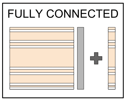
Basic fully connected layer


Introduction: deep neural networks
Basic fully connected network

Introduction: deep neural networks
Usual deep network

- Cascading linear and non-linear operations augments expressive power
- 7 millions parameters in our case
Introduction: deep neural networks
Training: vocabulary

Introduction: deep neural networks
Training: vocabulary

Introduction: deep neural networks
Training: vocabulary

Introduction: deep neural networks
Training: vocabulary
Introduction: deep neural networks
Training: the supervised approach

Introduction: deep neural networks
Training: the supervised approach

Introduction: deep neural networks
Training: the supervised approach

Introduction: deep neural networks
Training: the supervised approach

Introduction: deep neural networks
Training: the supervised approach

Introduction: deep neural networks
Training: the supervised approach
- $loss\leftarrow \sum_{(x,y)\in batch}cost\left(y_\Theta\left(x\right), y\right)$
- Update $\Theta$ to reduce the loss!
- We can compute $\frac{\partial loss}{\partial\Theta_{i}}$ for any parameter $\Theta_i$
- "The influence of $\Theta_i$ on the error"
- It's the gradient
- Computed through backpropagation
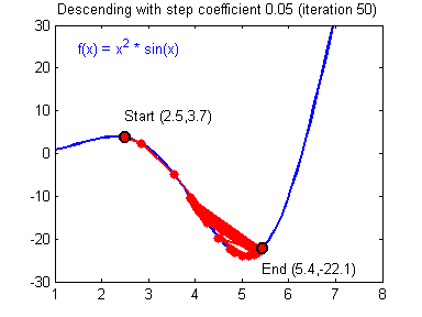
- A simple optimization: $\Theta_i\leftarrow \Theta_i - \lambda \frac{\partial loss}{\partial\Theta_{i}}$
- It's the stochastic gradient descent
- $\lambda$ is the learning rate
- Batching is important
There are many other optimization algorithms...
Introduction: modeling temporal data
colah's blog, Understanding LSTM Networks, 2015.
Introduction: modeling temporal data
From fully connected to the simple recurrent net

Introduction: modeling temporal data
From fully connected to the simple recurrent net

Introduction: modeling temporal data
From fully connected to the simple recurrent net

Introduction: modeling temporal data
From fully connected to the simple recurrent net

Introduction: modeling temporal data
The simple recurrent net

- $y_{t}=f\left(linear\left\{ x_{t},y_{t-1}\right\} \right)$
- Similar to a Markov model
- Exponential decay of information
- Vanishing or exploding gradient for training
- Limited for long-term dependencies
P. Huang, et al. "Deep learning for monaural speech separation". (2014) ICASSP.
Introduction: modeling temporal data
The long short term memory (LSTM)

Introduction: modeling temporal data
The long short term memory (LSTM)

Introduction: modeling temporal data
The long short term memory (LSTM)

Introduction: modeling temporal data
The bi-LSTM

- LSTM are causal systems
- Predicts future from past
Introduction: modeling temporal data
The bi-LSTM

- We can use anti-causal LSTM
- Different predictions!
Introduction: modeling temporal data
The bi-LSTM

- Independent forward and backward
- Outputs can be concatenated
- Outputs can be summed

Outline
Vanilla DNN for separation
- Model
- Spectrogram sampling
- Test
Vanilla DNN for separation: model


- One LSTM
- One fully connected
- 6 million parameters
- Implement the model in pytorch
Vanilla DNN for separation: spectrogram sampling

- Build a naive data sampler
- Start training the vanilla!
Vanilla DNN for separation: test

- Use the vanilla model for separation
Vanilla DNN for separation: evaluation

Outline
Choosing the right representation
- Input dimensionality reduction
- Fourier transforms parameters
- Standardization
Choosing the right representation: standardization

- Compensate different features scales
- Classical pre-processing
- Either dataset stats or trainable
Choosing the right representation: standardization


- Input/output scaling always lead to better loss
- Trainable is better than fixed
- Good loss needs scaling, but no influence on SDR
- We use scaling all the time
Choosing the right representation: Fourier transform

- Network is always fed 360ms of context
Choosing the right representation: Fourier transform

- Frames: 92ms=4096 samples @ 44k1kHz
- Overlap: 75%
- Long frames, large overlap
Choosing the right representation
Input dimensionality reduction

- Reduce number of parameters?
- From 6 million to 500k
- Fixed or trainable reduction
- Should we handcraft features?
Choosing the right representation
Input dimensionality reduction

- Reducing dimension
- Reduces model size
- Gives bettter performance
- Don't handcraft features, train them
Outline
DNN Structure: optimizing the vanilla net

- Network dimensions
- LSTM vs BLSTM
- Skip connection
DNN structure: network dimension

DNN structure: network dimension
The more parameters, the better


- Context length not so important
- LSTM unable to model long-term musical contexts?
- Hidden size (model dimension) has strong influene
- Large models are good
DNN structure: network dimension
The more parameters, the better, really?

- Moderate impact on SDR
- Strong impact on SIR
- Improves separation much
- But not a huge impact as in loss
- Loss on spectrograms is not audio quality
DNN structure: LSTM vs BLSTM

DNN structure: LSTM vs BLSTM


- Loss is similar
- BLSTM are better metric-wise
- In practice: BLSTM require the same context length at train and test
$\Rightarrow$ chop the data into batches at test time!
DNN structure: skip connection

- Should reduce vanishing gradient
- Much used in very deep nets
DNN structure: skip connection


- Improves loss slightly
- No effect on overall metrics
DNN structure: skip connection

- Better bass and drums
Recap: current structure for the baseline


Outline
Training
- Cost function
- Training tricks
- Data augmentation
- Sampling strategy
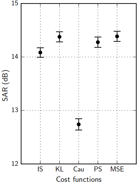
Training: the cost function jungle
 $loss=\sum_{b\in batch, f,t} d\left(Y_b\left(f,t\right),\hat{Y}_b\left(f,t\right)\right)$

- Wide variety of cost functions $d\left(a,b\right)$
- squared loss $\left|a-b\right|^2$
- absolute loss $\left|a-b\right|$
- Kullback Leibler loss $a\log\frac{a}{b}-a+b$
- Itakura Saito loss $\frac{a}{b}-\log\frac{a}{b}-1$
- Cauchy, alpha divergence, ...
- Applied on $Y$, $Y^2$, any $Y^\alpha$, $\log Y$, ...
- Theoretical groundings for all
C. Févotte, et al. "Algorithms for nonnegative matrix factorization with the β-divergence." Neural computation 23.9 (2011): 2421-2456.
A. Liutkus, et al. "Generalized Wiener filtering with fractional power spectrograms." (2015) ICASSP.
Training: the cost function jungle
A. Nugraha, et al. "Multichannel Audio Source Separation With Deep Neural Networks." TASLP 24.9 (2016): 1652-1664.
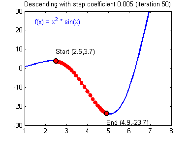
Training: learning rate and normalization
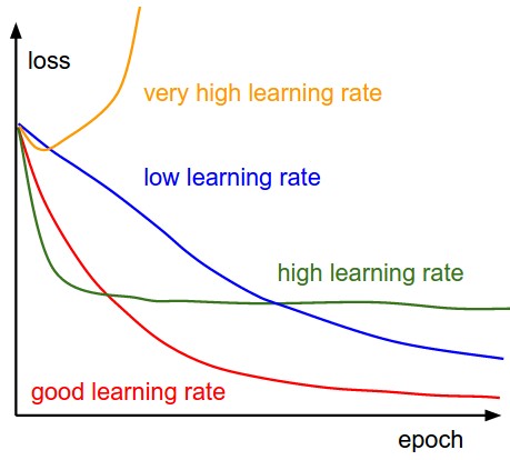
- We check for $\left[0.01, 0.001\right]$
Leonardo Araujo dos Santos, Artificial Intelligence, 2017.
Training: learning rate and normalization

Training: learning rate and normalization

- High learning rates don't work
- Keep default parameters for optim
Training: learning rate and normalization

- batchnorm fails in our case
- train batch: many songs
- test batch: one song
- layernorm forces matching
- test batch: normalized as in training
- batchnorm behaves wildly, avoid it

Training: learning rate and normalization

- Improves isolation: better SIR
- Adds distortion: worse SAR
Training: regularization with dropout
- Parts of the net randomly set to 0
- No unit should be critical: regularization
- Probabilistic interpretation
N Srivastava, et al. "Dropout: a simple way to prevent neural networks from overfitting". JMLR. (2014) 15(1), 1929-1958.
Training: regularization with dropout

- Regularization makes things worse
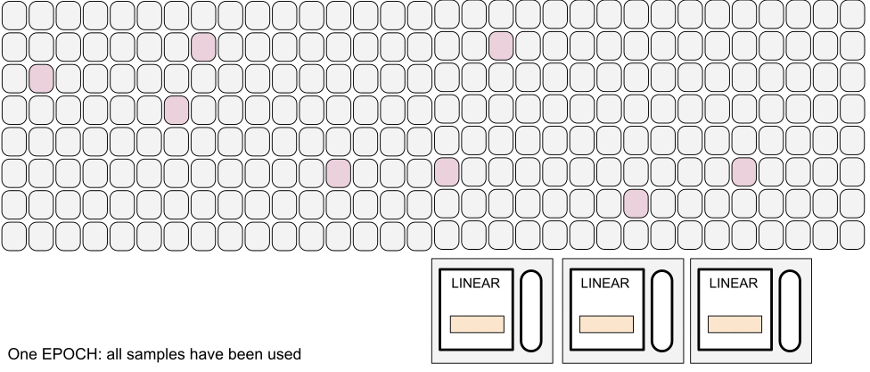
Training: sampling strategy
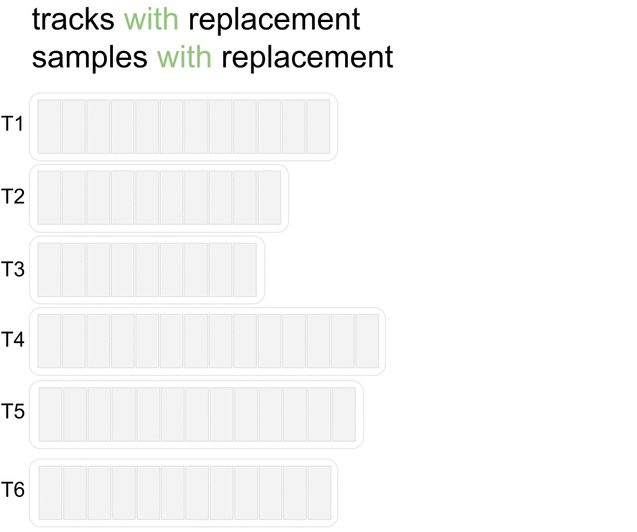
- Non unique tracks in batch
- Not all samples per epoch
Training: sampling strategy
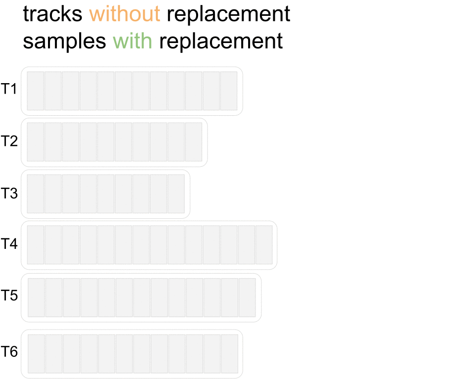
- Unique tracks in batch
- Not all samples per epoch
Training: sampling strategy
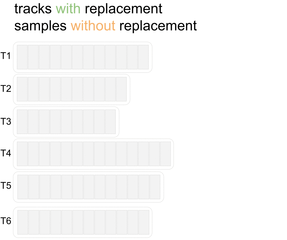
- Non unique tracks in batch
- All samples per epoch
Training: sampling strategy
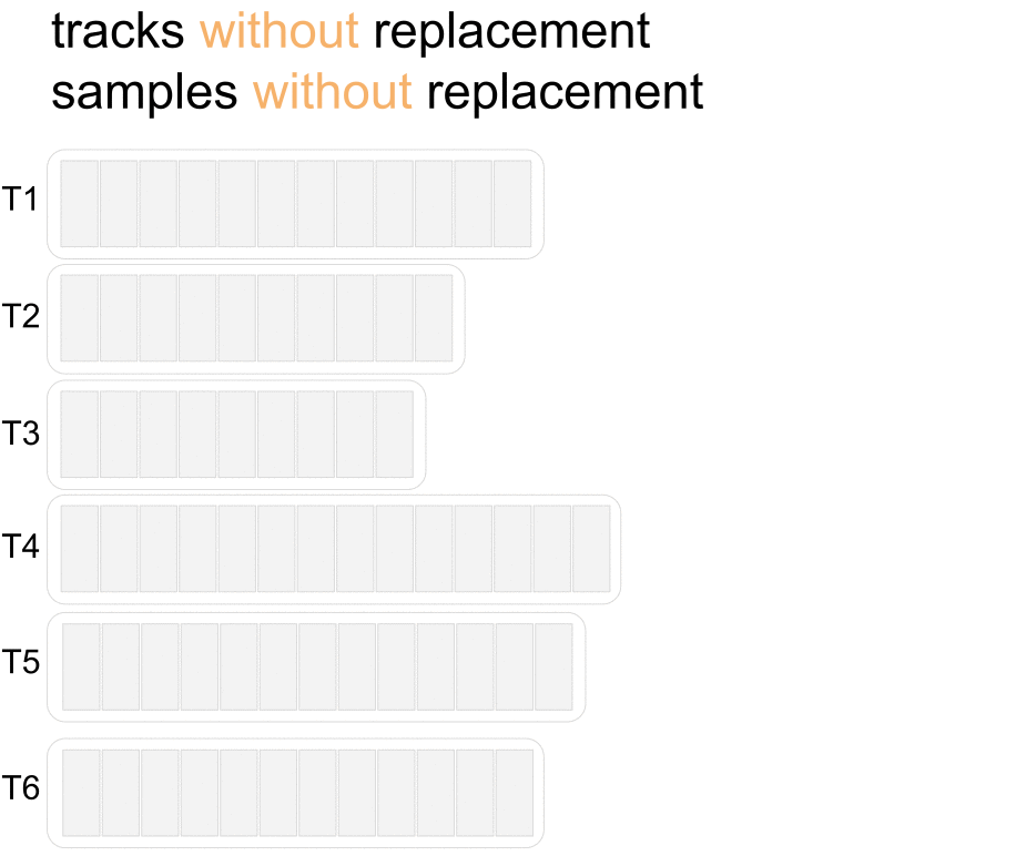
- Unique tracks in batch
- All samples per epoch
Training: sampling strategy
Hands on hierarchical sampling
- Implement the 4 strategies with pescador
- Apply they on spectrograms

Training: sampling strategy

- Unique tracks per batch is slower
- All samples per epoch is faster
B. Recht. "Beneath the valley of the noncommutative arithmetic-geometric mean inequality: conjectures, case-studies. and consequences." (2012). Technical report.
Training: data augmentation

- Basic augmentation: overlap samples within each track
- There are more advanced strategies
S. Uhlich, et al. "Improving music source separation based on deep neural networks through data augmentation and network blending." (2017) ICASSP.
Training: data augmentation

- Basic augmentation helps a bit (0.5dB)
- Not shown: new tracks are better!
Open Source Unmix (OSU) models


Outline
Testing
- Representation
- Mono filter tricks
- Multichannel Gaussian model
- The multichannel Wiener filter
- Testing: evaluation
Testing: representations
- The first source of poor results: inverse STFT!
- Verify perfect reconstruction
- Better: use established libraries, like
librosa,scipy...
Testing: mono filter tricks
Logit filters

- If the mask is 0.8... just put 1
- If the mask is 0.2... just put 0
- Cheap interference reduction
Multichannel Gaussian model

Multichannel Gaussian model

Multichannel Gaussian model

Multichannel Gaussian model

Multichannel Gaussian model

Multichannel Gaussian model

Testing: the multichannel Wiener filter

- Sources and mixtures are jointly Gaussian
- We observe the mix, what can we say about the sources?
Testing: the multichannel Wiener filter

Testing: the multichannel Wiener filter

Testing: the multichannel Wiener filter

Testing: the multichannel Wiener filter

Testing: the multichannel Wiener filter

Testing: the multichannel Wiener filter

Testing: the Expectation-Maximization algorithm

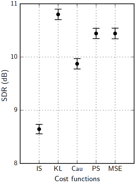
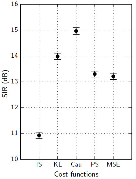
Testing: evaluation

Testing: evaluation

- Iterations improve SIR
$\Rightarrow$ greatly reduces interferences
- Iterations worsen SAR
$\Rightarrow$ introduces distortion
- logit has good SIR
$\Rightarrow$ cheap interference reduction

Testing: evaluation


Outline
Conclusion
- Resulting baseline
- What was kept out
- What is promising
- Ending remarks
Conclusion: the open source unmix


Conclusion: what was kept out
- Exotic representations

- Alternative structures
- The convolutional neural network (CNN)
- The U-NET
- The MM-densenet
- Deep clustering
- Generative approaches
- Generative adversarial nets
- (Variational) auto encoders
- Deep clustering
- Full grid search over parameters (fund us!)
- Advanced data augmentation (naive=+0.3dB SDR)
Conclusion: what is promising
More data
- More data
- Even more data
- Did we mention more data?
New approaches
- Structures with more parameters work better...
- Better signal processing helps
Engineering
- We got 3dB SDR improvement with no publishable contribution
$\Rightarrow$ evaluating the real impact of a contribution is difficult
Conclusion: ending remarks
- Convergence of signal processing, probability theory and DL
- Learning with limited amount of data
- Model long term dependency
- Representation learning for sound and music
- Exploiting knowledge domain, user interaction
- Unsupervised learning ?
Resources
- References and Software tools: sigsep.github.io
- SiSEC 2018 Website: sisec18.unmix.app

Deep Learning for Music Unmixing